What is a Signal?

Introduction to Signals and Systems

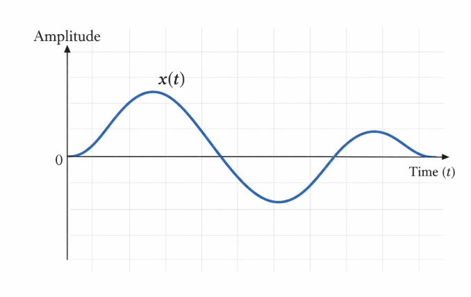
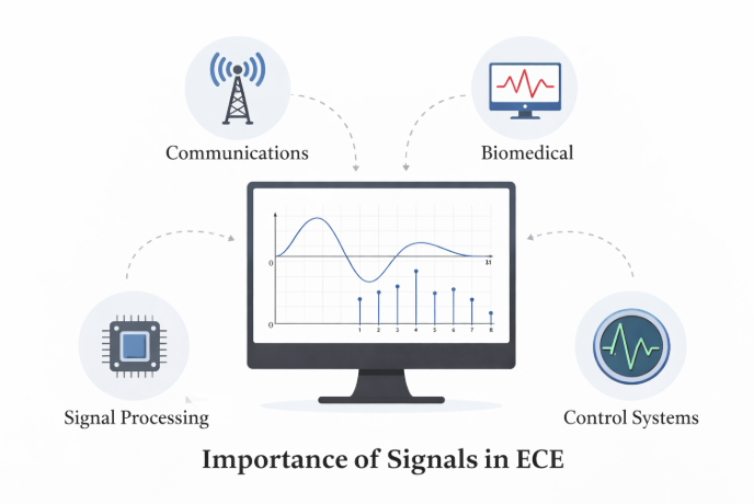
In engineering, a signal is a function that conveys information about the behavior or attributes of a physical system. Signals are fundamental to the analysis and design of communication, control, and signal processing systems.

Mathematically, a signal is expressed as a function of one or more independent variables. The most common case is a function of time.

Examples:

  • Continuous-time signal: x(t)
  • Discrete-time signal: x[n]

Signals may represent physical quantities such as sound pressure, voltage, temperature, or biological activity, and are analyzed using mathematical tools to extract useful information.

Examples of signals in engineering systems
Fig. 1. Examples of signals encountered in engineering systems.

Importance of Signals in Electronics Engineering

Why signals form the foundation of Electronics Engineering

Signals play a fundamental role in Electronics Engineering, as they provide a mathematical representation of physical phenomena such as voltage, current, and electromagnetic waves.

Nearly all electronic systems involve the generation, transmission, processing, or manipulation of signals. Through the study of signals, electronics engineers are able to analyze circuit behavior, design reliable systems, and interpret information accurately.

The study of signals is essential in the following areas of Electronics Engineering:

  • Communication Systems – analysis and transmission of analog and digital signals over electronic channels.
  • Analog and Digital Electronics – understanding signal behavior in amplifiers, filters, and logic circuits.
  • Digital Signal Processing – filtering, sampling, and spectral analysis of signals.
  • Embedded Systems – acquisition and processing of sensor and actuator signals using electronic hardware.
  • Biomedical Electronics – measurement and analysis of physiological signals such as ECG and EEG.

A strong understanding of signals enables electronics engineers to design efficient, stable, and high-performance electronic systems across a wide range of applications.

Role of signals in electronics engineering systems
Fig. 2. Role of signals in Electronics Engineering applications.

Classification of Signals

Categorizing signals based on their characteristics

Signals can be classified in several ways depending on their mathematical representation and physical behavior. These classifications are essential for analyzing electronic and signal processing systems.

1. Continuous-Time and Discrete-Time Signals

A continuous-time signal is defined for every value of time, whereas a discrete-time signal is defined only at specific instants.

t x(t)
Fig. 3. Continuous-time and discrete-time signals.
2. Periodic and Aperiodic Signals

A periodic signal repeats itself after a fixed interval, while an aperiodic signal does not exhibit repetition.

t x(t)
Fig. 4. Periodic (solid) and aperiodic (dashed) signals.
3. Energy and Power Signals

An energy signal has finite energy, whereas a power signal has finite average power over time.

t x(t)
Fig. 5. Energy (localized) and power (constant) signals.
4. Deterministic and Random Signals

A deterministic signal can be precisely described mathematically, while a random signal exhibits unpredictable behavior.

t x(t)
Fig. 6. Deterministic (smooth) and random (irregular) signals.

Continuous-Time and Discrete-Time Signals

Signal representation based on time

1. Continuous-Time Signals

A continuous-time signal is defined for every value of time. Such signals are common in analog electronic systems where voltage and current vary continuously.

The standard mathematical notation is x(t).

Fig. 7. Continuous-time signal x(t).
2. Discrete-Time Signals

A discrete-time signal is defined only at specific instants of time and is typically obtained through sampling.

Discrete-time signals are represented as x[n].

Fig. 8. Discrete-time signal x[n].

Operations on Signals

Continuous-time and discrete-time operations with reference signals

1. Time Shifting

CTS: y(t)=x(t−t₀)    DTS: y[n]=x[n−n₀]

Fig. 18a. CTS time shifting
Fig. 18b. DTS time shifting
2. Time Scaling

CTS: y(t)=x(at)    DTS: y[n]=x[⌊n/a⌋]

3. Time Reversal

CTS: y(t)=x(−t)    DTS: y[n]=x[−n]

4. Amplitude Scaling

CTS/DTS: y=A·x

5. Amplitude Shifting (DC Offset)

CTS/DTS: y=x+C

6. Signal Addition

CTS/DTS: y=x₁+x₂

7. Signal Multiplication

CTS/DTS: y=x₁·x₂